Zoo Pokedex Part 2: Hands on with Keras and Resnet50

Short Recap from Part 1

In the last blog post I briefly discussed the potential of using deep learning to build a zoo pokedex app that could be used to motivate zoo goers to engage with the animals and the information. We also discussed the imagenet competition and how deep learning has drastically changed the image recognition game. We went over the two main tricks that deep learning architectures do, namely convolutions and pooling, that allow such deep learning networks to perform extremely well. Last but not least we realized that all you have to do these days is to stand on the shoulders of giants by using the existing networks (e.g. Resnet50) to be able to write applications that have a similar state of the art precision. So finally in this blog post it’s time to put these giants to work for us.

Goal

The goal is to write an image detection app that will be able to distinguish animals in our zoo. Now for obvious reasons I will make our zoo really small, thus only containing two types of animals:

• Oryxes and
• LLamas (why there is a second L in english is beyond my comprehension).

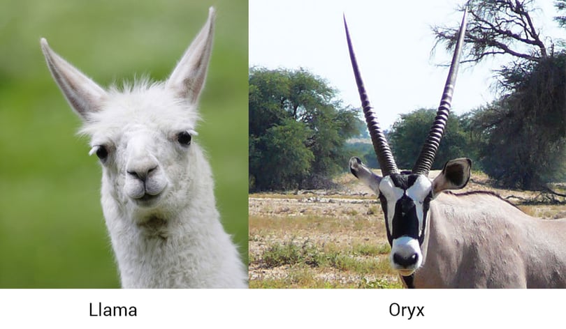
Why those animals? Well they seem fluffy, but mostly because the original imagenet competition does not contain these animals. So it represents a quite realistic scenario of a Zoo having animals that need to be distinguished but having existing deep learning networks that have not been trained for those. I really have picked these two kinds of animals mostly by random just to have something to show. (Actually I checked if the Zürich Zoo has these so i can take our little app and test it in real life, but that's already part of the third blog post regarding this topic)

Getting the data

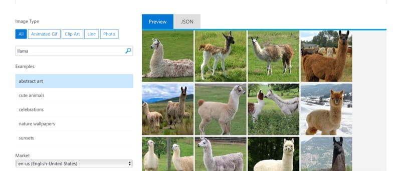
Getting data is easier than ever in the age of the internet. Probably in the 90ties I would have had to go to some archive or even worse take my own camera and shoot lots and lots of pictures of these animals to use them as training material. Today I can just ask Google to show me some. But wait - if you have actually tried using Google Image search as a resource you will realize that downloading their images in huge amounts is a pain in the ass. The image api is highly limited in terms of what you can get for free, and writing scrapers that download such images is not really fun. That's why I went to the competition and used Microsoft's cognitive services to download images for each animal.

Downloading image data from Microsoft

Microsoft offers quite a convenient image search API via their cogitive services. You can sign up there to get a free tier for a couple of days, which should be enough to get you started. What you basically need is an API Key and then you can already start downloading images to create your datasets.

# Code to download images via Microsoft cognitive api
require 'HTTParty'
require 'fileutils'

API_KEY = "##############"
SEARCH_TERM = "alpaka"
QUERY = "alpaka"
API_ENDPOINT  = "https://api.cognitive.microsoft.com/bing/v7.0/images/search"
FOLDER = "datasets"
BATCH_SIZE = 50
MAX = 1000

# Make the dir
FileUtils::mkdir_p "#{FOLDER}/#{SEARCH_TERM}"

# Make the request
headers = {'Ocp-Apim-Subscription-Key' => API_KEY}
query = {"q": QUERY, "offset": 0, "count": BATCH_SIZE}
puts("Searching for #{SEARCH_TERM}")
response = HTTParty.get(API_ENDPOINT,:query => query,:headers => headers)
total_matches = response["totalEstimatedMatches"]

i = 0
while response["nextOffset"] != nil && i < MAX
    response["value"].each do |image|
        i += 1
        content_url = image["contentUrl"]
        ext = content_url.scan(/^\.|jpg$|gif$|png$/)[0]
        file_name = "#{FOLDER}/#{SEARCH_TERM}/#{i}.#{ext}"
        next if ext == nil
        next if File.file?(file_name)
        begin
            puts("Offset #{response["nextOffset"]}. Downloading #{content_url}")
            r = HTTParty.get(content_url)
            File.open(file_name, 'wb') { |file| file.write(r.body) }
        rescue
            puts "Error fetching #{content_url}"
        end
    end
    query = {"q": SEARCH_TERM, "offset": i+BATCH_SIZE, "count": BATCH_SIZE}
    response = HTTParty.get(API_ENDPOINT,:query => query,:headers => headers)
end

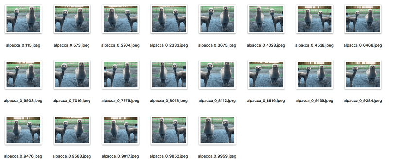
The ruby code above simple uses the API in batches and downloads llamas and oryxes into their separate directories and names them accordingly. What you don’t see is that I went through these folders by hand and removed images that were not really the animal, but for example a fluffy shoe, that showed up in the search results. I also de-duped each folder. You can scan the images quickly on your mac using the thumbnail preview or use an image browser that you are familiar with to do the job.

Problem with not enough data

Ignoring probable copyright issues (Am i allowed to train my neural network on copyrighted material) and depending on what you want to achieve you might run into the problem, that it’s not really that easy to gather 500 or 5000 images of oryxes and llamas. Also to make things a bit challenging I tried to see if it was possible to train the neural networks using only 100 examples of each animal while using roughly 50 examples to validate the accuracy of the networks.

Normally everyone would tell you that you need definitely more image material because deep learning networks need a lot of data to become useful. But in our case we are going to use two dirty tricks to try to get away with our really small collection: data augmentation and reuse of already pre-trained networks.

Image data generation

A really neat handy trick that seems to be prevalent everyday now is to take the images that you already have and change them slightly artificially. That means rotating them, changing the perspective, zooming in on them. What you end up is, that instead of having one image of a llama, you’ll have 20 pictures of that animal, just every picture being slightly different from the original one. This trick allows you to create more variation without actually having to download more material. It works quite well, but is definitely inferior to simply having more data.

We will be using Keras a deep learning library on top of tensorflow, that we have used before in other blog posts to create a good sentiment detection. In the domain of image recognition Keras can really show its strength, by already having built in methods to do image data generation for us, without having to involve any third party tools.

# Creating a Image data generator
train_datagen = ImageDataGenerator(preprocessing_function=preprocess_input,
    shear_range=0.2, zoom_range=0.2, horizontal_flip=True)

As you can see above we have created an image data generator, that uses sheering, zooming and horizontal flipping to change our llama pictures. We don’t do a vertical flip for example because its rather unrealistic that you will hold your phone upside down. Depending on the type of images (e.g. aerial photography) different transformations might or might not make sense.

# Creating variations to show you some examples
img = load_img('data/train/alpaka/Alpacca1.jpg')
x = img_to_array(img) 
x = x.reshape((1,) + x.shape)  
i = 0
for batch in train_datagen.flow(x, batch_size=1,
                          save_to_dir='preview', save_prefix='alpacca', save_format='jpeg'):
    i += 1
    if i > 20:
        break  # otherwise the generator would loop indefinitely

Now if you want to use that generators in our model directly you can use the convenient flow from directory method, where you can even define the target size, so you don’t have to scale down your training images with an external library.

# Flow from directory method
train_generator = train_datagen.flow_from_directory(train_data_dir,
    target_size=(sz, sz),
    batch_size=batch_size, class_mode='binary')

Using Resnet50

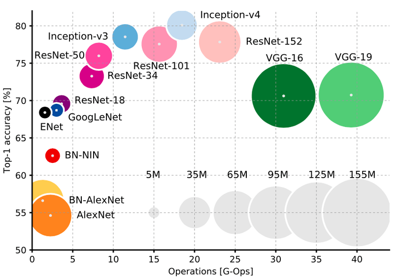
In order to finally step on the shoulder of giants we can simply import the resnet50 model, that we talked about earlier. Here is a detailed description of each layer and here is the matching paper that describes it in detail. While there are different alternatives that you might also use the resnet50 model has a fairly high accuracy, while not being too “big” in comparison to the computationally expensive VGG network architecture.

On a side note: The name “res” comes from residual. A residual can be understood a a subtraction of features that were learned from the input a leach layer. ResNet has a very neat trick that allows deeper network to learn from residuals by “short-circuiting” them with the deeper layers. So directly connecting the input of an n-th layer to some (n+x)th layer. This short-circuiting has been proven to make the training easier. It does so by helping with the problem of degrading accuracy, where networks that are too deep are becoming exponentially harder to train.

#importing resnet into keras
from keras.models import load_model
base_model = ResNet50(weights='imagenet')

As you can see above, importing the network is really dead easy in keras. It might take a while to download the network though. Notice that we are downloading the weights too, not only the architecture.

Training existing models

The next part is the exciting one. Now we finally get to train the existing networks on our own data. The simple but ineffective approach would be to download or just re-build the architecture of the successful network and train those with our data. The problem with that approach is, that we only have 100 images per class. 100 images per class are not even remotely close to being enough data to train those networks well enough to be useful.

Instead we will try another technique (which I somewhat stole from the great keras blog): We will freeze all weights of the downloaded network and add three final layers at the end of the network and then train those.

Freezing the base model

Why is this useful you might ask: Well by doing so we can freeze all of the existing layers of the resnet50 network and just train the final layer. This makes sense, since the imagenet task is about recognizing everyday objects from everyday photographs, and it is already very good at recognising “basic” features such as legs, eyes, circles, heads, etc… All of this “smartness” is already encoded in the weights (see the last blog post). If we throw these weights away we will lose these nice smart properties. But instead we can just glue another pooling layer and a dense layer at the very end of it, followed by a sigmoid activation layer, that's needed to distinguish between our two classes. That's by the way why it says “include_top=False” in the code, in order to not include the initial 1000 classes layer, that was used for the imagenet competition. Btw. If you want to read up on the different alternatives to the resnet50 you will find them here.

# Adding three layers on top of the network
base_model = ResNet50(weights='imagenet', include_top=False)
x = base_model.output
x = GlobalAveragePooling2D()(x)
x = Dense(1024, activation='relu')(x)
predictions = Dense(1, activation='sigmoid')(x)

Finally we can now re-train the network with our own image material and hope for it to turn out to be quite useful. I’ve had some trouble finding the right optimizer that had proper results. Usually you will have to experiment with the right learning rate to find a configuration that has an improving accuracy in the training phase.

#freezing all the original weights and compiling the network
from keras import optimizers
optimizer = optimizers.RMSprop(lr=0.00001, rho=0.9, epsilon=None, decay=0.0)
model = Model(inputs=base_model.input, outputs=predictions)
for layer in base_model.layers: layer.trainable = False
model.compile(optimizer=optimizer, loss='binary_crossentropy', metrics=['accuracy'])
model.fit_generator(train_generator, train_generator.n // batch_size, epochs=3, workers=4,
        validation_data=validation_generator, validation_steps=validation_generator.n // batch_size)

The training shouldn’t take long, even when you are using just a CPU instead of a GPU and the output might look something like this:

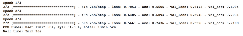
You’ll notice that we reached an accuracy of 71% which isn’t too bad, given that we have only 100 original images of each class.

Fine-tuning

One thing that we might do now is to unfreeze some of the very last layers in the network and re-train the network again, allowing those layers to change slightly. We’ll do this in the hope that allowing for more “wiggle-room”, while changing most of the actual weights, the network might give us better results.

# Make the very last layers trainable
split_at = 140
for layer in model.layers[:split_at]: layer.trainable = False
for layer in model.layers[split_at:]: layer.trainable = True
model.compile(optimizer=optimizers.RMSprop(lr=0.00001, rho=0.9, epsilon=None, decay=0.0), loss='binary_crossentropy', metrics=['accuracy'])    
model.fit_generator(train_generator, train_generator.n // batch_size, epochs=1, workers=3,
        validation_data=validation_generator, validation_steps=validation_generator.n // batch_size)

And indeed it helped our model to go from 71% accuracy to 82%! You might want play around with the learning rates a bit or maybe split it at a different depth, in order to tweak results. But generally I think that just adding more images would be the easiest way to achieve 90% accuracy.

Confusion matrix

In order to see how well our model is doing we might also compute a confusion matrix, thus calculating the true positives, true negatives, and the false positives and false negatives.

# Calculating confusion matrix
from sklearn.metrics import confusion_matrix
r = next(validation_generator)
probs = model.predict(r[0])
classes = []
for prob in probs:
    if prob < 0.5:
        classes.append(0)
    else:
        classes.append(1)
cm = confusion_matrix(classes, r[1])
cm

As you can see above I simply took the first batch from the validation generator (so the images of which we know if its a alpakka or an oryx) and then use the confusion matrix from scikit-learn to output something. So in the example below we see that 28 resp. 27 images of each class were labeled correctly while making an error in 4 resp. 5 images. I would say that’s quite a good result, given that we used only so little data.

#example output of confusion matrix
array([[28,  5],
       [ 4, 27]])

Use the model to predict images

Last but not least we can of course finally use the model to predict if an animal in our little zoo is an oryx or an alpakka.

# Helper function to display images
def load_image(img_path, show=False):

    img = image.load_img(img_path, target_size=(224, 224))
    img_tensor = image.img_to_array(img)                    # (height, width, channels)
    img_tensor = np.expand_dims(img_tensor, axis=0)         # (1, height, width, channels), add a dimension because the model expects this shape: (batch_size, height, width, channels)
    #img_tensor /= 255.                                      # imshow expects values in the range [0, 1]

    if show:
        plt.imshow(img_tensor[0]/255)                           
        plt.axis('off')
        plt.show()

    return img_tensor

# Load two sample images
oryx = load_image("data/valid/oryx/106.jpg", show=True)
alpaca = load_image("data/valid/alpaca/alpaca102.jpg", show=True)
model.predict(alpaka)
model.predict(oryx)

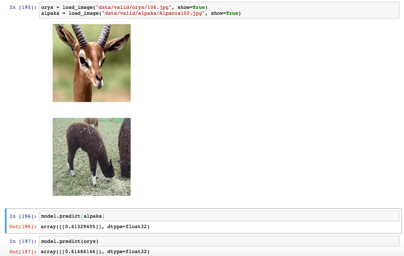
As you can see in the output, our model successfully labeled the alpaca as an alpaca since the value was less than 0.5 and the oryx as an oryx, since the value was > 0.5. Hooray!

Conclusion or What’s next?

I hope that the blog post was useful to you, and showed you that you don’t really need much in order to get started with deep learning for image recognition. I know that our example zoo pokedex is really small at this point, but I don’t see a reason (apart from the lack of time and resources) why it should be a problem to scale out from our 2 animals to 20 or 200.

On the technical side, now that we have a model running that’s kind of useful, it would be great to find out how to use it in on a smartphone e.g. the IPhone, to finally have a pokedex that we can really try out in the wild. I will cover that bit in the third part of the series, showing you how to export existing models to Apple mobile phones making use of the CoreML technology. As always I am looking forward to your comments and corrections and point you to the ipython notebook that you can download here.